Prepare your data and tools
Load the Packages that You Will Need
Packages are collections of R functions, data, and code that extend the basic functionality of R. R comes with a standard set of packages but there are many others available for download and installation. sdcMicro is an example of an add-on data package in R. In order to use it, you must first install it by running the function install.packages(). Once installed, you need to load package when you want to use it. For this session, you will need the packages sdcMicro, readxl, and tidyverse.
install.packages("sdcMicro")
library(readxl)
library(sdcMicro)
library(tidyverse)
Importing Data from Excel file
We will be working with an Excel file and so the next step is to pull our spreadsheet data into our RStudio workspace. You can download the data that we will be working with from this Google Drive folder. Please keep in mind that this data has been prepared for the purpose of this tutorial and should not be used for any other purpose. There are a few different ways to import data from Excel into R. Here, we will use the setwd() function to set our working directory to the folder where your data is saved. Then, using the read_excel() function, we will import the excel file and assign it to a new object (‘data’) as we have done below.
setwd ("/Users/username/sdcTutorial")
data <- read_excel("sdcTutorial_data.xlsx", sheet="settlementdata")
Dealing with Missing Values:
If you are working with a spreadsheet, before you import your data to R, it is worth taking the time to make sure that your data is well structured. This includes making sure that the first row in your spreadsheet is the header row, that you delete any comments in the dataset and deal with missing values. Missing values are represented in R by the NA symbol. In the language, NA is a special value whose properties are different from other values. In your data missing values may be represented as ‘N/A’, ‘na’, a blank cell and sometimes, unfortunately, all of the above. You will need to recode any missing values that are not coded as ‘NA’ to ‘NA’ before starting the SDC process (or doing any other analysis in R).Review Data Structure
Before you begin any analysis, you may want to review the data structure. This will tell you the type of object you have, how many rows (observations) and columns (variables) the object contains, the type of data in each column and the first few entries for each column. In the example below, you see that our data file has 7,005 records and 70 variables. You also learn the classes of the variables, numeric (num) and character (chr) respectively, and the first few values for those variables.
str(data)
tibble [7,005 × 70] (S3: tbl_df/tbl/data.frame)
 $ weights                                   : num [1:7005] 0.146 0.146 2.281 0.146 2.281 ...
 $ province                                  : chr [1:7005] "Balkh" "Balkh" "Balkh" "Balkh" ...
 $ district                                  : chr [1:7005] "Khuram Sarbagh" "Sar e Pul" "Pul e khumri" "Dawlatabad" ...
 $ community.damage                          : chr [1:7005] "Low community damage" "Low community damage" "Low community damage" "Low community damage" ...
 $ interviewer_sex                           : chr [1:7005] "Female" "Male" "Male" "Male" ...
Explore Relationship Between Variables
Now that you understand how the data is structured, you need to make sure that you understand exactly what each variable represents and explore the relationships between the variables. This is all part of your exploratory data analysis. This is how you get to know your dataset.
To make sure that you understand what is represented by each variable, we recommend looking at the data dictionary, the original questionnaire, or, if nothing else is available, reaching out to the data collector directly. Next, you can start to summarise the data to get a better understanding of what the whole dataset looks like. You might start by looking for outliers and doing some basic tabulation. For our assessment, we want to pay particular attention to common key variables like age, location and marital status.
One thing that you will notice exploring our data is that most of the likely key variables are categorical. Variables like locations, marital status, disability status have the class ‘chr’ (character or string). One exception is the head of household’s age which is a numeric variable (‘num’) and even age can be thought of as semi-continuous and treated as a categorical variable for the purpose of the disclosure risk assessment.
One way to explore the relationship between two categorical variables is to create a crosstab. You can do this using the function table().
table(data$hhh_ethnolinguistic_group,data$hhh_marital_status)
Divorced Married Single Widowed
Arab           192    6132    206      15
Aymaq            1      44      0       0
Baloch           3      39      3       0
Brahui           0       5      0       0
Gujjar           1      42      2       0
Hazara           1      42      2       0
Kyrgyz           0       5      0       0
Nuristani        1      44      0       0
Pamiri           1       4      0       0
Pashai           0      43      2       0
Pashtun          1      39      0       0
Tajik            1      44      0       0
Turkmen          1      42      2       0
Uzbek            2      40      3       0
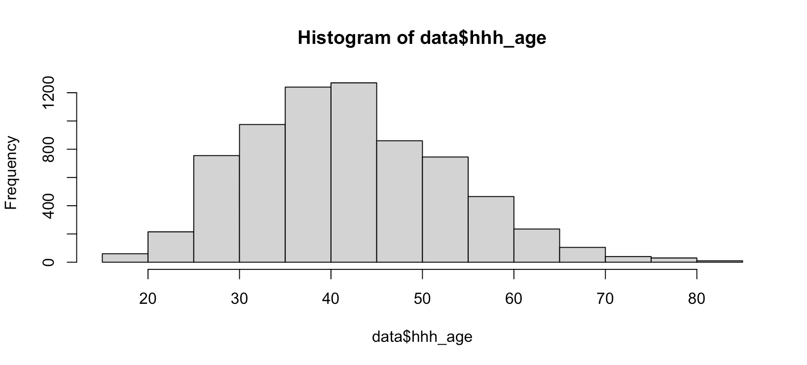
For numeric variables, such as age, you can use the hist() function to explore whether or not there are noticeable outliers.
Select key variables
The sdcMicro package is built around objects of class sdcMicroObj. In this section, we will walk through how to select key variables, set your sample weight variable and create a subset of your datafile. You will then use these new objects (selectedKeyVars, selectedWeights, and dataSub) as arguments of the function ‘createSdcObj()’ in order to create the sdcMicro object that you will use to assess the disclosure risk and apply disclosure control techniques.
Develop Disclosure Scenarios:
To develop a disclosure scenario, you will need to think through the motivations of any malicious actors, describe the data that they may have access to, and specify how this data and other publicly available data could be linked to your data and lead to disclosure. This requires you to make assumptions about what types of data and information others are likely to have access to. If you are not sure, we recommend creating multiple disclosure scenarios based on different assumptions and run the disclosure risk assessment on each.Select Weight & Key Variable
Now we need to select our key variables and sample weights. After exploring the data and developing disclosure risk scenarios, we identified the following key variables: district, head of household ethnolinguistic group, age, gender, marital status, and disability status and finally, total number of members of the household.
selectedKeyVars <- c('district', 'hhh_ethnolinguistic_group','hhh_marital_status', 'hhh_age', 'hhh_gender','hhh_disability', 'total_members')
selectedWeights <- c('weights')
Have your sample weights on hand:
In order to conduct the disclosure risk assessment, you will need the sample weights for the data that you are assessing. To find the sample weights you may need to review the data dictionary, the metadata or other documentation for the dataset. If you have no information about the sample weights, we recommend that you contact the data provider before conducting the assessment. However, if there are no available sample weights and you still want to conduct a disclosure risk assessment, you can treat the data as if all respondents are equally weighted and focus on k-anonymity as your measure of disclosure risk. Remember, k-anonymity does not take into account sample weights so the results will not be affected.
Create Subset of the Data File
Now that we know the keys variables that we want to focus on we are going to create a subset of the data file that contains only these variables and our sample weights. Before we create our subset of the data file, we need to convert the categorical variables from chr variables to factors. In our example, the categorical variables are district, ethnolinguistic group, marital status, gender and disability status. We will use the lapply() function to convert these variables from strings to factors and then create a subset of the data file.
## Create Subset of Data File
cols =  c('district', 'hhh_ethnolinguistic_group','hhh_marital_status', 'hhh_gender','hhh_disability')
data[,cols] <- lapply(data[,cols], factor)
subVars <- c(selectedKeyVars, selectedWeights)
subData <- data[,subVars]
Create sdcMicro Object
Finally, you are ready to create the sdcMicro object. Use the arguments of the function createSdcObj() to specify the data file (subData), the sample weights (selectedWeights) and the keyVars (selectedKeyVars). These are only a few of the arguments that are available. Read more about all of the arguments of this function in the sdcMicro documentaion.
## Create sdcMicro object
objSDC <- createSdcObj(dat=subData, keyVars = selectedKeyVars, weightVar = selectedWeights)
Run assessment & interpret results
Calculate Individual Risk, Sample and Population Frequency
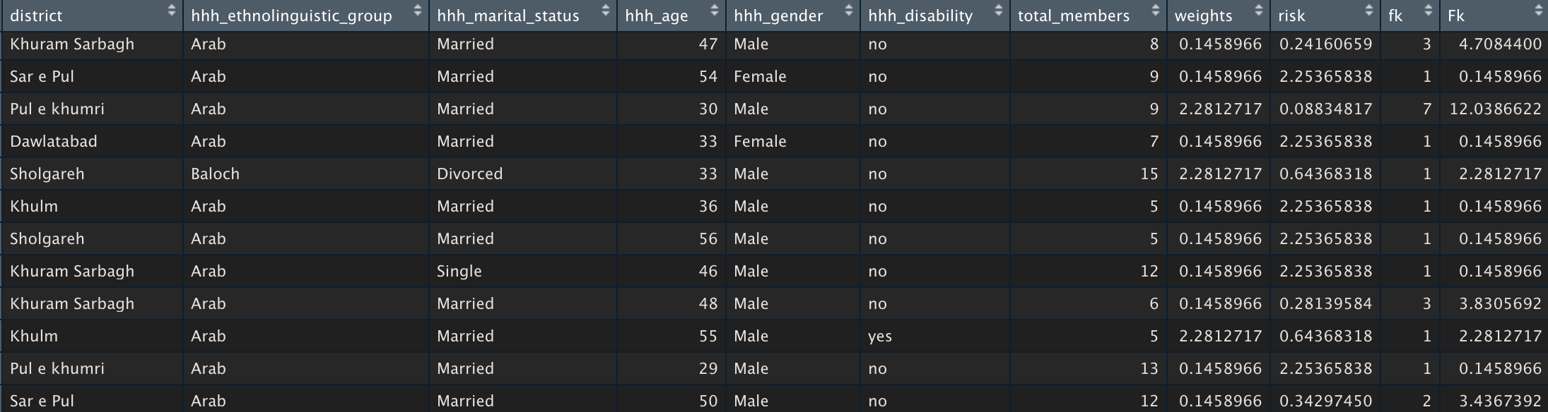
With your key variables selected and your sdcMicro object created, you are ready to run the assessment. First, we are going to create a new data frame that will combine the sample frequency (fk), population frequency (Fk) and individual risk measures to the subset of the data file that we created in step one (fileRes). Next, we will calculate the individual risk using the sdcMicro object that we just created. In order to make it easier to explore this data, we will assign its values to a new object (individual_risk) and then create a new data frame using the cbind() function.
individual_risk <- objSDC@risk$individual
indRisk_table <- cbind(subData,individual_risk)
View(indRisk_table)
The table will look like the table below with new columns for risk (individual disclosure risk), fk (sample frequency) and FK (population frequency).
Review K-Anonymity
Our next step is to review k-anonymity. Here, we will simply print 2-. 3-, and 5- anonymity.
## print K-anonimity
print(objSDC, type="kAnon")
Infos on 2/3-Anonymity:

Number of observations violating
  - 2-anonymity: 3255 (46.467%)
  - 3-anonymity: 4599 (65.653%)
  - 5-anonymity: 5873 (83.840%)

----------------------------------------------------------------------
As you can see, we have 3255 records that violate 2-anonymity. This is the number of unique keys in our data. For all public data shared on HDX, we review 3-anonymity and recommend that no record violates 3-anonymity. In this case, over 65% of the records violate K-anonymity. From here, it’s clear that we will need to apply statistical disclosure control before sharing this data publicly but before we do, we should review the global disclosure risk.
Calculate Global Risk
The final risk measure that we will calculate is the global risk measures. The global risk of re-identification is 99.24% (very high!). As we anticipated, we will need to apply disclosure control techniques before sharing this data widely.
## Print global risk
print(objSDC, "risk")
Risk measures:

Number of observations with higher risk than the main part of the data: 1914
Expected number of re-identifications: 6952.11 (99.24 %)
Managing data responsibly
Given this high risk of re-identification, we will have to apply statistical disclosure control techniques before sharing this data publicly. In this section, we will walk through how to use the sdcMicro package to apply two disclosure control techniques – global recoding and local suppression. Read more about these techniques and the other disclosure control techniques that can be applied in the sdcMicro documentation.
Apply Global Recoding
Global Recoding is a common disclosure control technique that involves reducing the number of values a given variable can take. It is an effective method for reducing the detail in the data while maintaining some of its analytical power. For numeric variables, recoding involves creating intervals or brackets (i.e. income or age). Recoding can also be used for categorical variables. For example, a geographic variable could be aggregated into groups like ‘north’, ‘south’, ‘east’ and ‘west’ or ‘urban’, ‘rural’ and ‘suburban’.
In the example below, the age variable is converted into ten age brackets with ten year increments and the total members variable is converted into five. After recoding each variable, you can use the table() function to see the distribution.
## Recode Age Variable
objSDC <- globalRecode(objSDC, column = c('hhh_age'), breaks = 10 * c(0:10))
table(objSDC@manipKeyVars$hhh_age)

  (0,10]  (10,20]  (20,30]  (30,40]  (40,50]  (50,60]  (60,70]  (70,80]
       0       60      970     2215     2130     1210      340       70
 (80,90] (90,100]
      10        0
## Recode Total Members Variables
objSDC <- globalRecode(objSDC, column = c('total_members'), breaks = 5 * c(0:5))
table(objSDC@manipKeyVars$total_members)

  (0,5]  (5,10] (10,15] (15,20] (20,25]
    566    4188    2059     182      10
Now that we have done this recoding, we want to determine the impact it has had reducing the global risk of disclosure. As you can see below, recoding these two variables reduces our global risk from 99.24% to 24.90%. A nearly 25% risk of disclosure is still quite high and so we will need apply additional disclosure control techniques before we share the data publicly.
print (objSDC,"risk")
Risk measures:

Number of observations with higher risk than the main part of the data:
  in modified data: 2010
  in original data: 1914
Expected number of re-identifications:
  in modified data: 1744.20 (24.90 %)
  in original data: 6952.11 (99.24 %)
Apply Local Suppression
If you want to further reduce the disclosure risk of your data, a next step might be to apply local suppression. WIth local suppression, individual values are suppressed (deleted) and replaced with NA (missing value). In the example below, local suppression is applied to achieve 3-anonymity. You can set K to whatever you’d like.
objSDC <- localSuppression(objSDC, k = 3, importance = NULL)
calcRisks(objSDC)
The input dataset consists of 7005 rows and 8 variables.
  --> Categorical key variables: district, hhh_ethnolinguistic_group, hhh_marital_status, hhh_age, hhh_gender, hhh_disability, total_members
  --> Weight variable: weights
----------------------------------------------------------------------


Information on categorical key variables:

Reported is the number, mean size and size of the smallest category >0 for recoded variables.
In parenthesis, the same statistics are shown for the unmodified data.
Note: NA (missings) are counted as separate categories!


              Key Variable Number of categories      Mean size
                  district                   21 (23)   264.696  (304.565)
 hhh_ethnolinguistic_group                   14 (14)   491.571  (500.357)
        hhh_marital_status                    5  (4)  1750.000 (1751.250)
                   hhh_age                    9 (62)   695.700  (112.984)
                hhh_gender                    2  (2)  3502.500 (3502.500)
            hhh_disability                    3  (2)  3502.000 (3502.500)
             total_members                    6 (23)  1398.800  (304.565)
 Size of smallest (>0)
                     5   (5)
                     2   (5)
                    15  (15)
                     7   (5)
                   175 (175)
                   579 (580)
                     7   (1)
----------------------------------------------------------------------


Infos on 2/3-Anonymity:

Number of observations violating
  - 2-anonymity: 0 (0.000%) | in original data: 3255 (46.467%)
  - 3-anonymity: 0 (0.000%) | in original data: 4599 (65.653%)
  - 5-anonymity: 83 (1.185%) | in original data: 5873 (83.840%)

----------------------------------------------------------------------


Local suppression:

                    KeyVar | Suppressions (#) | Suppressions (%)
                  district |              917 |           13.091
 hhh_ethnolinguistic_group |              123 |            1.756
        hhh_marital_status |                5 |            0.071
                   hhh_age |               48 |            0.685
                hhh_gender |                0 |            0.000
            hhh_disability |                1 |            0.014
             total_members |               11 |            0.157
----------------------------------------------------------------------
In our example, 13% of the district variable’s values have been suppressed means that 13% of the district names have been replaced with NA. This is something that you will want to consider when evaluating the information loss. If district level information is critical for downstream users and the suppression of 13% of the districts would severely limit their ability to conduct analysis, then it may be more interesting to share the data less widely, using, for example, an information sharing protocol.
Reassess Disclosure Risk
Now that we have applied global recoding and local suppression, we again want to reassess the disclosure risk before applying any additional disclosure control. Ultimately, we have reduced the risk of disclosure from 99.24% to 3.93%. This would still be too high to share on HDX.
print(objSDC,"risk")
Risk measures:

Number of observations with higher risk than the main part of the data:
  in modified data: 566
  in original data: 1914
Expected number of re-identifications:
  in modified data: 275.39 (3.93 %)
  in original data: 6952.11 (99.24 %)
Quantify Information Loss
Before we decide to further reduce the risk of disclosure, we are going to quantify the information loss to decide whether it makes sense or if we should be exploring other ways to share the data. There are quite a few methods for quantifying information loss and in this tutorial, we will not go into these in too much detail.
Below are two tables showing the distribution of the ethnolinguistic group variable before and after treatment (local suppression). Overall, for this variable, 123 values were replaced with missing values and all but one of these come from non-arab groups. For example, you can see in the second table that all 5 Pamiri responses were suppressed. We could do the same of the other variables to see what impact the information loss will have on different forms of analysis. In the end, there is no objective way to determine whether the information loss. We have to assess this in regards to the needs of downstream users.
table(objSDC@origData[, c('hhh_ethnolinguistic_group')])

     Arab    Aymaq    Baloch    Brahui    Gujjar    Hazara    Kyrgyz Nuristani
     6545        45        45         5        45        45         5        45
   Pamiri    Pashai   Pashtun     Tajik   Turkmen     Uzbek
        5        45        40        45        45        45


table(objSDC@manipKeyVars[, c('hhh_ethnolinguistic_group')])

     Arab    Aymaq    Baloch    Brahui    Gujjar    Hazara    Kyrgyz Nuristani
     6544        37        24         3        34        32         2        35
   Pamiri    Pashai   Pashtun     Tajik   Turkmen     Uzbek
        0        37        29        39        35        31
From here, we could decide that the level of information loss is tolerable and apply additional statistical disclosure techniques to further reduce the risk of disclosure (at least below the 3% threshold for sharing data on HDX). Alternatively, we could decide that the information loss is too high, especially in regards to a few of our key variables, and instead explore other ways to share the data safely. To learn more about responsible data sharing, we recommend that you read the Centre’s Draft Guidelines on Data Responsibility.